We’re usually putzing around in a 3 dimensional space, perceiving the 4th dimension of time as something we’re moving forward through. Attempts to explain our reality, however, have intriguingly and disturbingly given rise to the possibility of higher dimensions. Superstring Theory, for example, posits 10 dimensions to provide a unifying framework between general relativity and quantum mechanics. M-Theory, on the other hand, posits 11 dimensions, and Bosonic String Theory a daunting 26 dimensions! In machine learning we work in even higher dimensions to model data. For example, Google’s BERT projects words on to 768 or 1024 dimensional spaces in order to model human language.

What do these higher dimensions “look like”? The short answer is that to beings such as ourselves, i.e., mostly 3D with some limited 4D perception: very weird! Visualizing these higher dimensions in the traditional sense doesn’t seem possible for us, but we can still get insight into these spaces through mathematics. Frustratingly, many of these insights break from our usual 2D or 3D intuitions. As Thomas Banchoff wrote, “All of us are slaves to the prejudices of our own dimension.”

Read on to mathematically “see” some weird stuff in high dimensions.

Sources: This post is compiled using notes from CMU, Cornell, and UC Davis with some additional figures and exposition for my own understanding.

Warmup
Sphere
Cube
Gaussians

Warmup

Consider a d−dimensional unit square. If were to place n points inside the square such that each coordinate for each point is drawn uniformly at random from the interval [0,1], what can we say about the distribution of distances between points?

Our usual intuition might be that the points will be spread out somewhat evenly. This holds true in our familiar 2D and 3D spaces. However, something different happens in higher dimensions.

Consider that the distance between any two points X=(xi,…,xd) and Y=(y1,…,yd) is defined as ,

D=|X−Y|=√d∑i=1(xi−yi)2

where for each dimension i∈{1,…,d},

xii.i.d∼Unif(0,1)yii.i.d∼Unif(0,1)

Then (xi−yi)2 are i.i.d random variables for all i, and D2 is a summation of independent random variables.

So in high dimensions, the Law of Large Numbers applies and D2 converges to its expected value. The distances are then concentrated around a mean! However, in lower dimensions (like the 2D and 3D we’re perceptually accustomed to), D2 is pre-convergence and the distances are still spread out.

Sphere

Consider a d− dimensional sphere of unit radius centered at the origin: {(x1,x2,⋯,xd):∑di=1x2i≤1}

Compute surface area and volume
Volume goes to zero
Volume is near the equator
Volume is a narrow annulus

Compute surface area and volume

The surface area A(d) and the volume V(d) of a unit-radius sphere in d dimensions are given by A(d)=2πd2Γ(d2) and V(d)=πd2d2Γ(d2) where Γ is the Gamma functions.

Proof

Cartesian Coordinates

First, lets recall that in 3-dimensions a sphere of radius a is defined as x2+y2+z2=a2. In order to compute its volume we consider the region x2+y2+z2≤a2.

• Solving for z gives: −√a2−x2−y2≤z≤√a2−x2−y2
• The projection of the sphere onto the xy−plane when z=0 is the circle x2+y2=a2. Then solving for y within the desired region gives: −√a2−x2≤y≤√a2−x2
• −a≤x≤a

Thus, the volume of the sphere can be computed as:

V(3)=∫a−a∫√a2−x2−√a2−x2∫√a2−x2−y2−√a2−x2−y21dzdydx Extending this formula to a d-dimensional sphere of radius 1 gives:

V(d)=∫1−1∫√1−x21−√1−x21⋯∫√1−x21−⋯−x2d−1−√1−x21−⋯−x2d−1 dxd dxd−1⋯dx1

Polar Coordinates

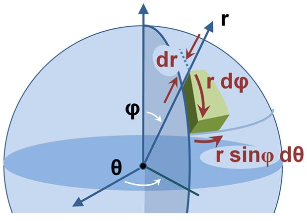
In 3-dimensions, a sphere of radius a is defined as all points where 0≤ϕ≤π, 0≤θ≤2π, and 0≤r≤a. Then the volume of the sphere can be computed as,

V(3)=∫π0∫2π0∫a0r2sin(ϕ)drdθdϕ Using the concept of a solid angle to further simplify the integral by allowing us to write it over a coordinate free ‘direction’. Let dΩ=sin(ϕ)dθdϕ be the surface area of the infinitismal piece of the solid angle S3 of the sphere.

Then,

V(3)=∫S3∫ar=0r2dΩdr Extending this formula to a d-dimensional sphere of unit radius gives:

V(d)=∫Sd∫1r=0rd−1 dr dΩ=(∫Sd dΩ)(∫1r=0rd−1 dr)(Variables are independent)=1d∫Sd dΩ=1dA(d)(i)

A Trick

Consider a different problem: I(d) def =∫∞−∞∫∞−∞⋯∫∞−∞e−(x21+x22+⋯+x2d)dxd⋯dx2 dx1

This can be computed in both Cartesian and Polar coordinates. They will be equated to solve our problem.

Cartesian: I(d)=∫∞−∞∫∞−∞…∫∞−∞e−(x21+x22+⋯+x2d)dxd⋯dx2 dx1=[∫∞−∞e−(x1)2 dx1]d(independent coordinates across same range)=(√π)d=πd2 Polar: I(d)=∫∞−∞∫∞−∞…∫∞−∞e−(x21+x22+⋯+x2d)dxd⋯dx2 dx1=∫Sd∫∞−∞e−r2rd−1 dr dΩ(Definition of sphere+ change to polar)=(∫Sd dΩ)(∫∞−∞e−r2rd−1 dr)(Independent variables)=A(d)2∫∞0e−ttd−1212√t dt (Let t=r2≥0, so r=√t, dr=12√t dt ) =A(d)∫∞0e−ttd2−1 dt=A(d)Γ(d2)(Definition of Γ function).

Then by equating the solution for I(d) in cartesian and polar coordinates,

A(d)=2πd2Γ(d2)

Finally, using equation (i),

V(d)=πd2d2Γ(d2)

More generally, the surface area and volume equations for a d−sphere of radius r are,

Ar(d)=2πd2Γ(d2)rd−1=A(d)rd−1andVr(d)=πd2Γ(d2+1)rd=V(d)rd

Volume goes to zero

By Stirling’s Formula, Γ(d2)≈√2πd/2(d/2e)d2=√4πd(d2e)d2

So, the denominator of V(d) grows faster than its numerator since dd2 grows much faster than πd2,. Thus,

V(d)→0 as d→∞

Volume is near the equator

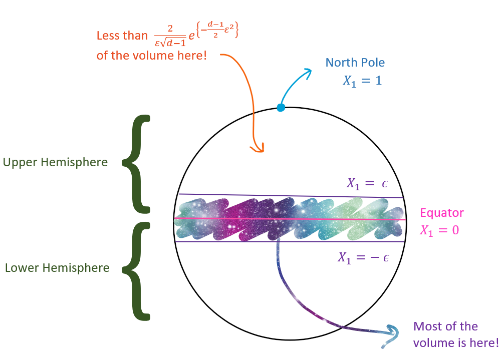
Without loss of generality, pick any of the d poles of the sphere as the North Pole, say the pole along x1. Then the North Pole is x1=1.

Define the equator as the (d−1) dimensional sphere: {x||x∣≤1,x1=0}. This is formed by the intersection of the x1=0 plane with the d−sphere. It has volume V(d−1). Note that, in 3-dimensions this is (familiarly) a circle.

The equator divides the sphere into two hemispheres, or d-dimensional half spheres, one upper and one lower.

Consider a plane x1=ϵ slightly above the x1=0 plane, for some ϵ>0. Less than 2ε√(d−1)e−d−12ε2 fraction of the volume in the upper hemisphere lies above the x1=ϵ plane. This value drops exponentially with ϵ2 as ϵ increases and d goes to infinity. Same is true for volume below x1=−ϵ in the lower hemisphere.

Proof

Without loss of generality we will show the bound for the upper hemisphere.

Define the region T as the portion of the sphere above the x1=ϵ plane: T={x||x∣≤1,x1≥ε}. Then,

Upper bound on proportion of volume above ϵ= Upper bound of Vol(T) Lower bound of Vol( hemisphere )= Upper bound of Vol(T) Lower bound of 12Vol(d)

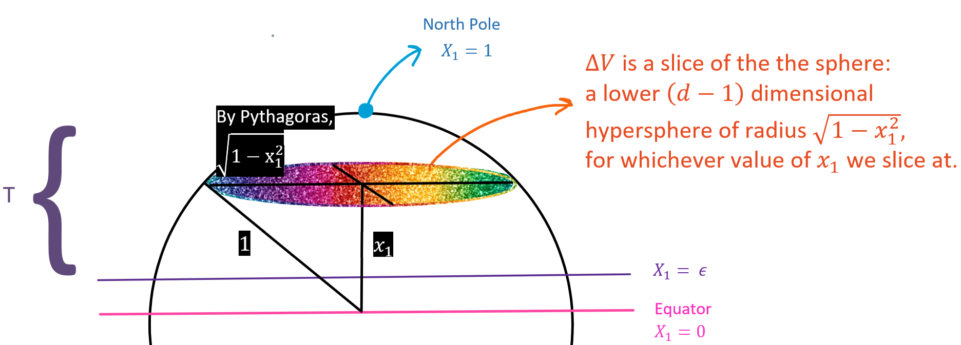
Vol(T)=∫1ϵΔV dx1(ΔV is a cross-sectional slice )=∫1ϵV(d−1)rd−1 dx1(Volume of (d−1) dimensional sphere of radius r)=V(d−1)∫1ϵ(1−x1)d−12 dx1(r=√1−x21)≤V(d−1)∫1ϵe−x21d−12 dx1(Lemma 1)≤V(d−1)∫∞ϵe−x21d−12 dx1(e−x21d−12≥0∀x1∈[ϵ,∞])≤V(d−1)∫∞ϵx1ϵe−x21d−12 dx1(x1ϵ≥1∀x1∈[ϵ,∞])=V(d−1)−2ϵd−12∫∞ϵe−x21d−12 d(−x21d−12)(Subst: u=−x21d−12;du=−2d−12x1dx1)=V(d−1)ϵ(d−1)e−x21d−12|∞ϵ=1ϵ(d−1)e−d−12ϵ2V(d−1) 12V(d)=∫10V(d−1)rd−1 dx1=V(d−1)∫10(1−x21)d−12 dx1≥V(d−1)∫1√d−10(1−x21)d−12 dx1≥V(d−1)∫1√d−10(1−d−12x21)dx1( Lemma 2)≥V(d−1)∫1√d−10(1−d−121d−1)dx1(t2≤1d−1∀x1∈[0,1√d−1])=V(d−1)∫1√d−1012=12√d−1V(d−1)

Thus,

Upper bound on proportion of volume above ϵ=1ϵ(d−1)e−d−12ϵ2V(d−1)12√d−1V(d−1)=2ε√(d−1)e−d−12ε2

Volume is a narrow annulus

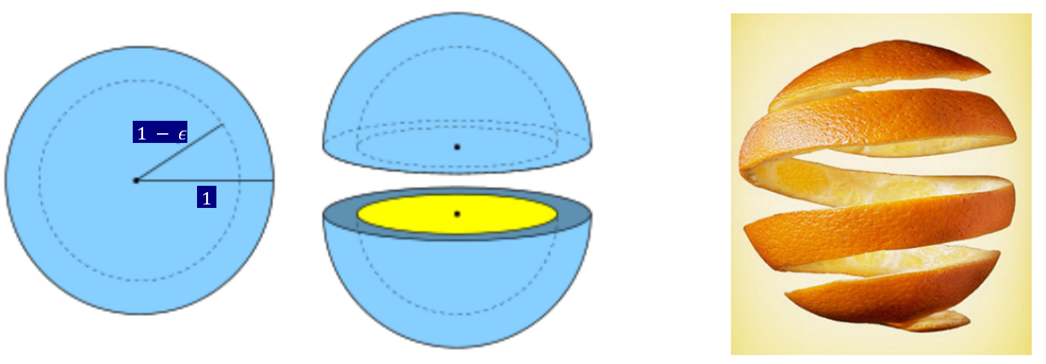
The ratio of the volume of a d−sphere of radius 1−ϵ to one with unit raduis is,

V1−ϵ(d)V1(d)=(1−ε)dV(d)V(d)=(1−ε)d This ratio →0 as d→∞. So in high dimensions, all of the volume of the sphere is concentrated in a narrow annulus at the surface.

Cube

Consider a d−dimensional cube with unit-length sides centered at the origin.

• As d increases, the volume remains constant at 1d=1.
• However, the maximum distant between points, i.e. from one vertex to another, keeps increasing as √d. Eg. the distance between the vertex at (12,…,12) and (−12,…,−12) is √d∗(12+12)2=√d

This is in interesting contrast to what we saw of the d−dimensional sphere of unit radius we saw earlier where,

• As d increases the volume →0, and
• The maximum distance between two points given by the diameter remains constant at 2r=2.

The relationship between the unit-length hypercube and unit-radius hypersphere as d increases is shown below.

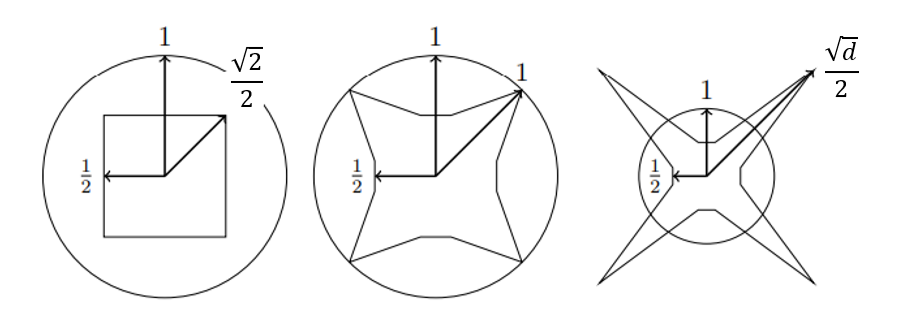
• For d=2, the cube is completely inside the sphere. Distance from origin to a vertex=√(12)2+(12)2=√22≅0.707

• For d=4, the vertices of the cube lies exactly on the boundary of the sphere since the distance of from the origin to a vertex of the cube=√(12)2+(12)2+(12)2+(12)2=1

• For any higher dimensions, the vertices of the cube exceed the confines of the sphere! However, there are still points of the cube that remain within the sphere (eg. (12,0,…,0)). So the high dimensional hypercube ends up with a “spiky” shape with distance from origin to a vertex=√d∗(12)2=√d4=√d2

Other weird stuff

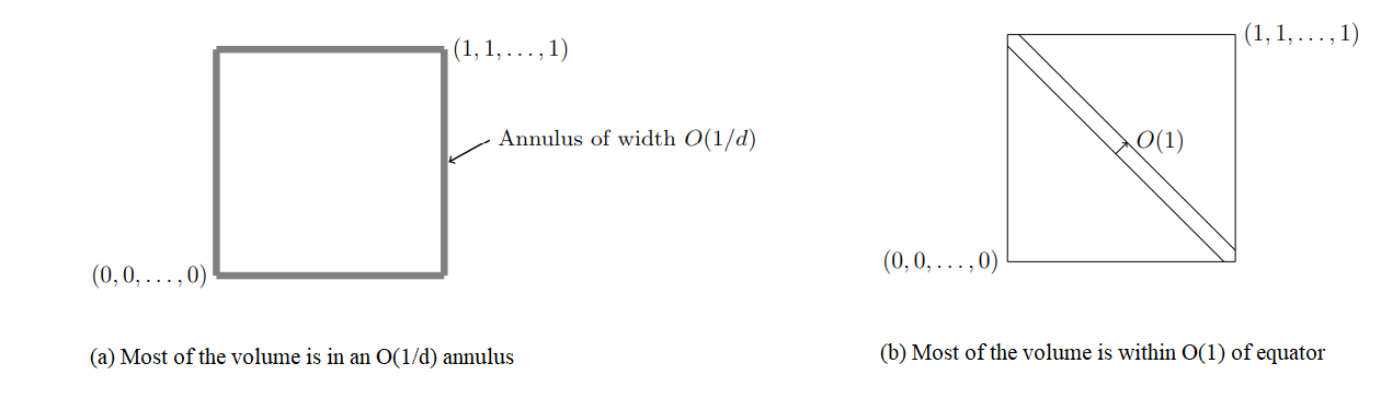
• Most of the volume is within a narrow O(1/d) annulus
• Most of the volume is concentrated about the equator, defined as

Gaussians

• For a d-dimensional spherical Gaussian of variance 1 , all but 4c2e−c2/4 fraction of its mass is within the annulus √d−1−c≤r≤√d−1+c for any c>0

• Ω(d1/4) separation is required to separate means of d-dimensional spherical Gaussian of variance 1.