Box Embeddings: Paper Overviews
Tamanna Hossain-Kay / 2021-11-09
Geometric embeddings can be used to represent transitive asymmetric relationships. Box-embeddings are n-dimensional hyperrectangles that can represent such relationships by containment.
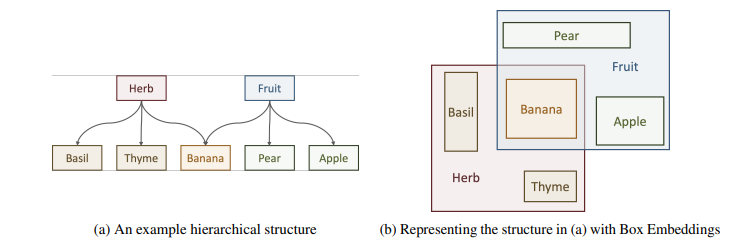
Formally, a “box” is defined as a Cartesian product of closed intervals, \[ \begin{aligned} B(\theta) &=\prod_{i=1}^{n}\left[z_{i}(\theta), Z_{i}(\theta)\right] \\ &=\left[z_{1}(\theta), Z_{1}(\theta)\right] \times \cdots \times\left[z_{n}(\theta), Z_{n}(\theta)\right]\\ &=[x_{m,1},x_{M,1}]\times \cdots \times [x_{m,n},x_{M,n}] \end{aligned} \]
Parameterization: \(\theta\) may be the output from a neural network
Python package: Box Embeddings: An open-source library for representation learning using geometric structures
In order to learn box-embeddings, intersections and volumes of boxes need to be computed. This can be done in a few different ways:
- Hard Intersection + Hard Volume: Probabilistic Embedding of Knowledge Graphs with Box Lattice Measures (Vilnis et al., 2018)
- Hard Intersection + Soft Volume: Smoothing the Geometry of Probabilistic Box Embeddings (Li et al., 2018)
- Gumbel Intersection + Bessel Approx. Volume: Improving Local Identifiability in Probabilistic Box Embeddings (Dasgupta et al., 2020)
Read on for brief overviews of each method.
Probabilistic Embedding of Knowledge Graphs with Box Lattice Measures
Authors: Luke Vilnis, Xiang Li, Shikhar Murty, Andrew McCallum; University of Massachusetts Amherst
Method: Hard Intersection, Hard Volume
Defining Box operations
\[ \begin{array}{l} x \wedge y=\perp \text { if } x \text { and } y \text { disjoint, else } \\ x \wedge y=\prod_{i}\left[\max \left(x_{m, i}, y_{m, i}\right), \min \left(x_{M, i}, y_{M, i}\right)\right] \\ x \vee y=\prod_{i}\left[\min \left(x_{m, i}, y_{m, i}\right), \max \left(x_{M, i}, y_{M, i}\right)\right] \end{array} \]
Note,
- While boxes are closed under intersection they’re not closed under union.
- \((x \wedge y)= (x \cap y\)), but \((x \vee y) > (x \cup y)\)
Volume can be computed as,
\[ Vol(B(\theta)) = \prod_{i} \max (x_{M, i}-x_{m, i},0)=\prod_{i} m_h(x_{M, i}-x_{m, i})\]
where \(m_h\) is the standard hinge function.
Volume can be interpreted as probability. For a concept \(c\) associated with box \(B(\theta)\),
\[P(c) = Vol (B(\theta))\]
Learning WordNet
The transitive reduction of the WordNet noun hierarchy contains 82,114 entities and 84,363 edges.
The learning task is an edge classification task. Given a pair of nodes \((h, t)\), the probability of existence of the edge \(h_{i} \rightarrow t_{i}\) is computed as \[ P\left(h_{i} \rightarrow t_{i}\right)= P(h_i|t_i)=\frac{P(h_i \cap t_i)}{P(t_i)}=\frac{\operatorname{Vol}\left(\mathrm{B}\left(\theta_{h_{i}}\right) \cap \mathrm{B}\left(\theta_{t_{i}}\right)\right)}{\operatorname{Vol}\left(\mathrm{B}\left(\theta_{t_{i}}\right)\right)} \]
Gold label: Existence \(\left(h_{i} \rightarrow t_{i}\right) \iff P(h_i|t_i)=1\)
Loss: Cross-entropy
Surrogate Intersection: When boxes do not intersect, the joint probability is 0 so parameters cannot be updated. In this case, a lower bound is used:
\[ \begin{aligned} p(a \cap b) &=p(a)+p(b)-p(a \cup b) \\ & \geq p(a)+p(b)-p(a \vee b) \end{aligned} \]
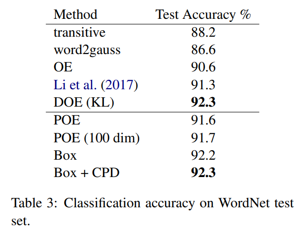
WordNet Results
Box-embeddings perform better than baselines in terms of classification accuracy. Refer to paper for details on baseline models.
Smoothing the Geometry of Probabilistic Box Embeddings
Authors: Xiang Li, Luke Vilnis,Dongxu Zhang, Michael Boratko, Andrew McCallum; University of Massachusetts Amherst
Method: Hard Intersection, Soft Volume
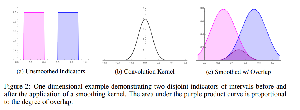
As mentioned in the previous paper (Vilnis et al., 2018), the gradient cannot flow when boxes disjoint. Vilnis et al., 2018 address this issue using a surrogate intersection probability. Here an alternative is proposed using using a Gaussian convolution with the original boxes to smooth the box edges into density functions.
Define boxes as indicator functions of intervals. Volume of boxes can then be expressed as integrals over the products of the indicator functions. Consider the 1D case for ease of exposition and results will generalize to higher dimensions.
The volume of the intersection of two boxes representing the intervals \(x=[a,b]\) and \(y=[c,d]\) (representing the joint probability between intervals) can be expressed as,
\[ p(\mathbf{x} \wedge \mathbf{y})=\int_{\mathbb{R}} \mathbb{1}_{[a, b]}(x) \mathbb{1}_{[c, d]}(x) d x \]
The smoothed version is,
\[ p_{\phi}(\mathbf{x} \wedge \mathbf{y})=\int_{\mathbb{R}} f\left(x ; a, b, \sigma_{1}^{2}\right) g\left(x ; c, d, \sigma_{2}^{2}\right) d x \]
where,
\[ f\left(x ; a, b, \sigma^{2}\right)=\mathbb{1}_{[a, b]}(x) * \phi\left(x ; \sigma^{2}\right)=\int_{\mathbb{R}} \mathbb{1}_{[a, b]}(z) \phi\left(x-z ; \sigma^{2}\right) d z=\int_{a}^{b} \phi\left(x-z ; \sigma^{2}\right) d z \]
and \[ \phi\left(z ; \sigma^{2}\right)=\frac{1}{\sigma \sqrt{2 \pi}} e^{\frac{-z^{2}}{2 \sigma^{2}}} \quad\text{(Gaussian PDF)} \]
Integral Solution:
\[ \begin{aligned} p_{\phi}(\mathbf{x} \wedge \mathbf{y}) &=\sigma\left(m_{\Phi}\left(\frac{b-c}{\sigma}\right)+m_{\Phi}\left(\frac{a-d}{\sigma}\right)-m_{\Phi}\left(\frac{b-d}{\sigma}\right)-m_{\Phi}\left(\frac{a-c}{\sigma}\right)\right) \end{aligned} \] where \(\sigma=\sqrt{\sigma_{1}^{2}+\sigma_{2}^{2}}\), \(\text{soft}(x)=\log (1+\exp (x))\) is the softplus function, the integral of the logistic sigmoid, and \(\rho=\frac{\sigma}{1.702}\)
Proof
Let \(\tau:=\frac{1}{\sqrt{\sigma_{1}^{2}+\sigma_{2}^{2}}}\), and note the identity from (Jebara et al., 2004; Vilnis & McCallum, 2015):
\[ \int_{\mathbb{R}} \phi\left(x-\mu_{1} ; \sigma_{1}^{2}\right) \phi\left(x-\mu_{2} ; \sigma_{2}^{2}\right) d x=\phi\left(\mu_{1}-\mu_{2} ; \sigma_{1}^{2}+\sigma_{2}^{2}\right) \]
Then, \[ \begin{aligned} p_{\phi}(\mathbf{x} \wedge \mathbf{y}) &=\int_{\mathbb{R}} \int_{a}^{b} \phi\left(x-y ; \sigma_{1}^{2}\right) d y \int_{c}^{d} \phi\left(x-z ; \sigma_{2}^{2}\right) d z d x \quad\text{Definition $f,g$}\\ &=\int_{a}^{b} \int_{c}^{d}\int_{\mathbb{R}}\phi\left(x-y ; \sigma_{1}^{2}\right) \phi\left(x-z ; \sigma_{2}^{2}\right) dx dy dz \quad\text{Fubini's Theorem}\\ &=\int_{c}^{d} \int_{a}^{b} \phi\left(y-z ; \tau^{-2}\right) d y d z \quad\text{(Jebara et al., 2004; Vilnis & McCallum, 2015)} \\ &=\int_{c}^{d} \int_{a}^{b} \Phi^{\prime}(\tau(y-z)) \tau dy dz \quad\text{Chain Rule; $\Phi$ is the standard normal CDF}\\ &=\int_{c}^{d} \Phi(\tau(b-z))-\Phi(\tau(a-z)) d z \\ &=\frac{-1}{\tau}\left(m_{\Phi}(\tau(b-d))-m_{\Phi}(\tau(a-d))-m_{\Phi}(\tau(b-c))+m_{\Phi}(\tau(a-c))\right) \end{aligned} \] Then with \(\sigma=\tau^{-1}\), \[ p_{\phi}(\mathbf{x} \wedge \mathbf{y})=\sigma\left(m_{\Phi}\left(\frac{b-c}{\sigma}\right)+m_{\Phi}\left(\frac{a-d}{\sigma}\right)-m_{\Phi}\left(\frac{b-d}{\sigma}\right)-m_{\Phi}\left(\frac{a-c}{\sigma}\right)\right) \]
Approximation
Multiplication of Gaussian-smoothed indicators have the property \(f^{2} \neq f\) so for cases \(\rho>0\),
- Idempotency requirement of bounded lattices is violated: \(a \wedge a=a \vee a=a\)
- Practically then if we are to treat the outputs of \(p_{\phi}\) as probabilities, the consequence is \[ p_{\phi}(\mathbf{x} \mid \mathbf{x})=\frac{p_{\phi}(\mathbf{x}, \mathbf{x})}{p_{\phi}(\mathbf{x})}=\frac{p_{\phi}(\mathbf{x} \wedge \mathbf{x})}{p_{\phi}(\mathbf{x})} \neq 1 \]
So we will approximate to get a version that is idempotent.
\[ \begin{aligned} p_{\phi}(\mathbf{x} \wedge \mathbf{y}) & \approx\left(\rho \operatorname{soft}\left(\frac{b-c}{\rho}\right)+\rho \operatorname{soft}\left(\frac{a-d}{\rho}\right)\right)-\left(\rho \operatorname{soft}\left(\frac{b-d}{\rho}\right)+\rho \operatorname{soft}\left(\frac{a-c}{\rho}\right)\right)\\ & \approx (\operatorname{soft}(b-c) \vee \operatorname{soft}(a-d)) \wedge(\operatorname{soft}(b-d) \vee \operatorname{soft}(a-c))=\operatorname{soft}(b \wedge d-a \vee c)\\ &=\operatorname{soft}(b \wedge d-a \vee c) \end{aligned} \]
The first approximation follows from the approximation of \(\Phi\) by a logistic sigmoid given in Bowling et al. (2009).
However, it is still not idempotent except in the zero-temperature limit. Since as \(\rho\) goes to zero, we recover the original formula with the hinge function which is idempotent, \[ \begin{aligned} p_{\phi}(\mathbf{x} \wedge \mathbf{y}) &=\lim _{\rho \rightarrow 0}\left(\rho \operatorname{soft}\left(\frac{b-c}{\rho}\right)+\rho \operatorname{soft}\left(\frac{a-d}{\rho}\right)\right)-\left(\rho \operatorname{soft}\left(\frac{b-d}{\rho}\right)+\rho \operatorname{soft}\left(\frac{a-c}{\rho}\right)\right) \\ &=\left(m_{h}(b-c)+m_{h}(a-d)\right)-\left(m_{h}(b-d)+m_{h}(a-c)\right) \\ &=m_{h}(b \wedge d-a \vee c) \quad\text{hinge function on an interval} \end{aligned} \]The limit
(From Wolfram Alpha) Two-sided limit does not exist.
Limit from the left: \(\lim _{\rho \rightarrow 0^{-}} \rho \log \left(1+\exp \left(\frac{y}{\rho}\right)\right)=0\) for \(y>0\)
Limit from the right: \(\lim _{\rho \rightarrow 0^{+}} \rho \log \left(1+\exp \left(\frac{y}{\rho}\right)\right)=y\) for \(y>0\)
The second approximation is needed to get a similar idempotent property when using the softplus fuinction as when using the hinge function,
\[ \left(m_{h}(b-c)+m_{h}(a-d)\right)-\left(m_{h}(b-d)+m_{h}(a-c)\right)=m_{h}(b \wedge d-a \vee c) \]
\[ (\operatorname{soft}(b-c) \vee \operatorname{soft}(a-d)) \wedge(\operatorname{soft}(b-d) \vee \operatorname{soft}(a-c))=\operatorname{soft}(b \wedge d-a \vee c) \]
Normalization
But finally, because softplus upper-bounds the hinge function, it is capable of outputting values that are greater than 1 , and therefore must be normalized.
Thus, in the multi-dimensional case we have:
\[ \begin{aligned} p(\mathbf{x}) & \approx \prod_{i} m_{\mathrm{soft}}^{(i)}\left(x_{M, i}-x_{m, i}\right)\\ p(\mathbf{x}, \mathbf{y}) & \approx \prod_{i} m_{\mathrm{soft}}^{(i)}\left(x_{M, i} \wedge y_{M, i}-x_{m, i} \vee y_{m, i}\right) \end{aligned} \]
where,
\[ m_{\mathrm{soft}}^{(i)}(x)=\frac{\operatorname{soft}\left(\frac{x}{\rho}\right)}{\operatorname{soft}\left(\frac{G_{m}-G_{m}}{\rho}\right)} \]
and \(\left(G_{m}^{(i)}, G_{M}^{(i)}\right)\)= Global minimum and maximum in \(i^{th}\) dimension.
WordNet Results
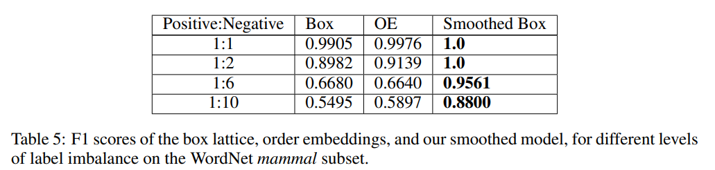
Sparsity is increased (positive:negative ratio increased) in the data to create more disjoint cases. In sparser regimes, the smoothed box greatly outperforms the baselines (original hard box, and OE).
Improving Local Identifiability in Probabilistic Box Embeddings
Authors: Shib Sankar Dasgupta, Michael Boratko, Dongxu Zhang, Luke Vilnis, Xiang Lorraine Li, Andrew McCallum; University of Massachusetts, Amherst
Method: Gumbel Intersection, Bessel Approx. Volume
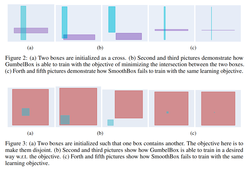
Both of the above proposed methods can have problems with local indentifiability since many different configurations of boxes can lead to the same joint probability value. This can lead to pathological parameter settings during train (Figure 2c; Figure 3c).
The method proposed here defines box edges as random variable, which leads to probabilities as expected volumes. This densifies the gradient of joint probabilities.
Gumbel Distribution
Since computing intersections of boxes involves computing minima and maxima, a min-max stable distribution is chosen: Gumbel distribution. This means that the maximum of multiple Gumbel random variables also follows a Gumbel distribution (MaxGumbel), and the minimum of multiple Gumbel random variables also follows a Gumbel distribution (MinGumbel).
Specifically,
If \(X_i \sim \operatorname{MaxGumbel}\left(\mu_{x_i}, \beta\right)\) then \[ \begin{aligned} \max (X_i) &\sim \operatorname{MaxGumbel}\left(\beta \ln \left(\sum_i e^{\frac{\mu_{x_i}}{\beta}}\right), \beta\right)\\ &= \operatorname{MaxGumbel}\left(\beta \operatorname{LogSumExp}(\frac{\mu_{x_i}}{\beta})\right) \end{aligned} \] and if \(X_i \sim \operatorname{MinGumbel}\left(\mu_{x}, \beta\right)\), then \[ \begin{aligned} \min (X_i) &\sim \operatorname{MinGumbel}\left(-\beta \ln \left( \sum_i e^{-\frac{\mu_{x_i}}{\beta}}\right), \beta\right)\\ &= \operatorname{MinGumbel}\left(-\beta \operatorname{LogSumExp}(-\frac{\mu_{x_i}}{\beta})\right) \end{aligned} \]
Gumbel-box process
For a probability space \(\left(\Omega_{\text {Box }}, \mathcal{E}, P_{\text {Box }}\right)\), with \(\Omega_{\mathrm{Box}} \subseteq \mathbb{R}^{d}\), the Gumbel-box process is generated as \[ \begin{aligned} \beta & \in \mathbb{R}_{+}, \quad \mu^{i, \vee} \in \Omega_{\mathrm{Box}} \quad \mu^{i, \wedge} \in \Omega_{\mathrm{Box}} \\ X_{j}^{i, \wedge} & \sim \operatorname{MaxGumbel}\left(\mu_{j}^{i, \wedge}, \beta\right), \quad X_{j}^{i, \vee} \sim \operatorname{MinGumbel}\left(\mu_{j}^{i, \vee}, \beta\right) \\ \operatorname{Box}\left(X^{i}\right) &=\prod_{j=1}^{d}\left[X_{j}^{i, \wedge}, X_{j}^{i, \vee}\right], \quad X^{i}=\mathbb{1}_{\operatorname{Box}\left(X^{i}\right)} \\ x^{1}, \ldots, x^{n} & \sim P\left(X^{1}, \ldots, X^{n}\right) \end{aligned} \] For a uniform base measure on \(\mathbb{R}^{d}\), each \(X^{i}\) is distributed according to \[ X^{i} \sim \operatorname{Bernoulli}\left(\prod_{j=1}^{d}\left(X_{j}^{i, \vee}-X_{j}^{i, \wedge}\right)\right) \]Intersection
\[ \begin{aligned} x \wedge y &= \prod_i [\mu_{\max _{X^{t} \in T} X_{j}^{t, \vee}}, \mu_{\min _{X^{t} \in T} X_{j}^{t, \wedge}}]\\ &= \prod_i \left[\beta \operatorname{LogSumExp}\left(\frac{\mu_{j}^{t, \vee}}{\beta}\right), -\beta \operatorname{LogSumExp}_{X^{t} \in T}\left(-\frac{\mu_{j}^{t, \wedge}}{\beta}\right)\right] \end{aligned} \]
Volume Calculation
The expected length of an interval \([X, Y]\) where \(X \sim \operatorname{MaxGumbel}\left(\mu_{x}, \beta\right)\) and \(Y \sim \operatorname{MinGumbel}\left(\mu_{y}, \beta\right)\) is given by \[ \mathbb{E}[\max (Y-X, 0)]=2 \beta K_{0}\left(2 e^{-\frac{\mu_{y}-\mu_{x}}{2 \beta}}\right) \] where \(K_{0}\) is the modified Bessel function of second kind, order \(0 .\)
Proof
\[ \begin{aligned} E[\max (Y-X, 0)]=& \iint_{\{y>x\}}(y-x) f_{\wedge}\left(y ; \mu_{y}\right) f_{\vee}\left(x ; \mu_{x}\right) d x d y \\ =& \int_{-\infty}^{\infty} \int_{-\infty}^{y} y f_{\wedge}\left(y ; \mu_{y}\right) f_{\vee}\left(x ; \mu_{x}\right) d x d y-\\ & \int_{-\infty}^{\infty} \int_{x}^{\infty} x f_{\wedge}\left(y ; \mu_{y}\right) f_{\vee}\left(x ; \mu_{x}\right) d y d x \\ =& \int_{-\infty}^{\infty} y f_{\wedge}\left(y ; \mu_{y}\right) F_{\vee}\left(y ; \mu_{x}\right) d y-\\ & \int_{-\infty}^{\infty} x f_{\vee}\left(x ; \mu_{x}\right)\left(1-F_{\wedge}\left(x ; \mu_{y}\right)\right) d x \\ & \int_{-\infty}^{\infty} y f_{\wedge}\left(y ; \mu_{y}\right) F_{\vee}\left(y ; \mu_{x}\right) d y-\\ =& \int_{-\infty}^{\infty} x f_{\vee}\left(x ; \mu_{x}\right) F_{\vee}\left(-x ;-\mu_{y}\right) d x \end{aligned} \] We note that this is equal to \[ E_{Y}\left[Y \cdot F_{\vee}\left(Y ; \mu_{x}\right)\right]-E_{X}\left[X \cdot F_{\vee}\left(-X ;-\mu_{y}\right)\right] \] however this calculation can be continued, combining the integrals, as \(=\int_{-\infty}^{\infty} z f_{\wedge}\left(z ; \mu_{y}\right) F_{\mathrm{\vee}}\left(z ; \mu_{x}\right)-z f_{\mathrm{V}}\left(z ; \mu_{x}\right) F_{\mathrm{V}}\left(-z ;-\mu_{y}\right) d z\) We integrate by parts, letting \(u=z, \quad d v=\frac{1}{\beta}\left(e^{\frac{\pi-\mu_{\mu}}{\beta}}-e^{-\frac{\tilde - \mu_{-}}{\beta}}\right) \exp \left(-e^{\frac{\pi-\mu_{\nu}}{\beta}}-e^{-\frac{\tilde - \mu_{2}}{\beta}}\right) d z\), \(d u=d z, \quad v=-\exp \left(-e^{\frac{x-\mu_{\mu}}{\beta}}-e^{-\frac{x-\mu \pi}{\beta}}\right)\) where the \(d v\) portion made use of the substitution \[ w=e^{\frac{\tilde - \mu_{\mu}}{\beta}}+e^{-\frac{-\mu-\mu}{\beta}}, \quad d w=\frac{1}{\beta}\left(e^{\frac{\tilde - \mu_{\mu}}{\beta}}-e^{-\frac{\tilde{-\mu}}{\beta}}\right) d z \] We have, therefore, that (12) becomes \[ =-\left.z \exp \left(-e^{\frac{z-\mu_{\mu}}{\beta}}-e^{-\frac{\tilde - \mu}{\beta}}\right)\right|_{-\infty} ^{\infty}+\int_{-\infty}^{\infty} \exp \left(-e^{\frac{x-\mu_{\mu}}{\beta}}-e^{-\frac{\tilde - \mu}{\beta}}\right) d z \] The first term goes to \(0 .\) Setting \(u=\frac{z-\left(\mu_{y}+\mu_{z}\right) / 2}{\beta}\) the second term becomes \[ \beta \int_{-\infty}^{\infty} \exp \left(-e^{\frac{\mu_{x}-\mu_{u}}{2 \bar{\beta}}}\left(e^{u}+e^{-u}\right)\right) d u=2 \beta \int_{0}^{\infty} \exp \left(-2 e^{\frac{\mu_{x}-\mu_{u}}{2 \bar{N}}} \cosh u\right) d u \] With \(z=2 e^{\frac{\mu_{x}-\mu_{y}}{2, S}}\), this is a known integral representation of the modified Bessel function of the second kind of order zero, \(K_{0}(z)\) [4, Eq. 10.32.9], which completes the proof of proposition 1 .
Let \(m(x)=\mathbb{E}[max(x,0)]=2 \beta K_{0}\left(2 e^{-\frac{x}{2 \beta}}\right) .\) Then the expected volume is, \[ \begin{aligned} &\mathbb{E}\left[\prod _ { i = 1 } ^ { d } \operatorname { m a x } \left(\min _{X^{t} \in T} X_{j}^{t, \wedge}-\max _{X^{t} \in T} X_{j}^{t, \vee}, 0\right)\right] \\ &= \prod _ { i = 1 } ^ { d } \mathbb{E}\left[ \operatorname { m a x } \left(\min _{X^{t} \in T} X_{j}^{t, \wedge}-\max _{X^{t} \in T} X_{j}^{t, \vee}, 0\right)\right] \quad\text{rearrange product and expectation}\\ &=\prod _ { i = 1 } ^ { d } m(\min _{X^{t} \in T} X_{j}^{t, \wedge}-\max _{X^{t} \in T} X_{j}^{t, \vee}) \quad\text{definition of m}\\ &=\prod_{i=1}^{d} 2 \beta K_0\left(2 e ^{ \frac{-\beta \operatorname{LogSumExp}_{X^{t} \in T}\left(-\frac{\mu_{j}^{t, \wedge}}{\beta}\right)-\beta \operatorname{LogSumExp}\left(\frac{\mu_{j}^{t, \vee}}{\beta}\right)}{2\beta}} \right) \quad\text{solution for m} \end{aligned} \] where \(T\) is a set of variables taking the value 1, and \(\mu^{t, \wedge}\) and \(\mu^{t, \vee}\) are the vectors of location parameters for the minimum and maximum coordinates of a \(\operatorname{Box}\left(X^{t}\right)\).
Approximation
Computing conditional probabilities exactly requires the conditional expectation, \(\mathbb{E}\left[P\left(x^{i}, x^{j}, Z\right) / P\left(x^{j}, Z\right)\right]\) which is intractable since it is a quotient. Instead, we approximate it by its first-order Taylor expansion, which takes the form of a ratio of two simple expectations: \(\mathbb{E}\left[P\left(x^{i}, x^{j}, Z\right)\right] / \mathbb{E}\left[P\left(x^{j}, Z\right)\right]\)
Softplus Approximation
Due to extreme similarity of the exact volume to the softplus function, the following approximation is used:
\[ m(x) \approx \beta \log (1+\exp (x / \beta-2 \gamma) \]
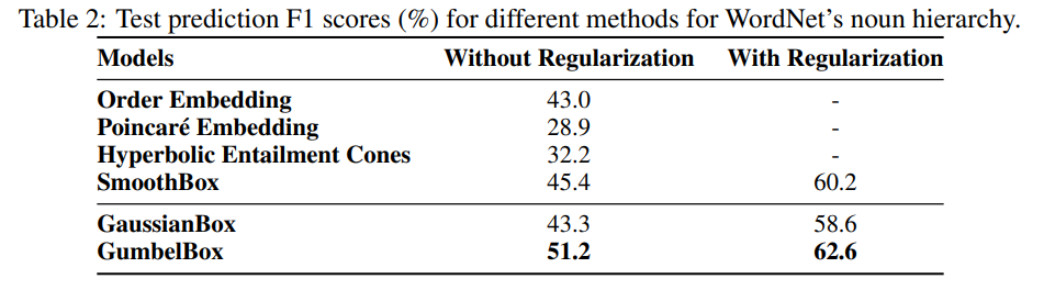
WordNet Results
Gumbel boxes perform better than baselines on WordNet’s noun hierarchy in terms of F1 score. Refer to paper for details on baseline models.