I came across the Orthogonal Procrustes technique when reading the paper Diachronic Word Embeddings Reveal Statistical Laws of Semantic Change. It was used to align word embeddings from different runs of SVD (Singular Value Decomposition) and SGNS (Skipgram with Negative Sampling), since they can both result in arbitrary orthogonal transformations of word vectors.

So what is Orthogonal Procrustes?

Problem
Solution
Proof of Solution
Example

Problem

Given two matrices \(A\), \(B\) find a matrix \(R\) for mapping \(A\) to \(B\). Specifically,

\[ R=\arg \min _{\Omega}\|\Omega A-B\|_{F} \quad \text { subject to } \quad \Omega^{T} \Omega=I \] where \(\|\cdot\|_{F}\) denotes the Frobenius norm.

Solution

Let \(M=BA^T\) and \(M=U \Sigma V^T\) be its factorization (SVD). Then the matrix for mapping \(A\) to \(B\) is \(R=UV^T\).

Proof of Solution

This proof is based on the one found in Wikipedia: Orthogonal Procrustes problem with additional exposition for my own understanding:

\[\begin{aligned} R &=\arg \min _{\Omega}\|\Omega A-B\|_{F}^{2} \\ &=\arg \min _{\Omega}\langle\Omega A-B, \Omega A-B\rangle_F &&\text{Frobenius innter product induces the norm}\\ &=\arg \min _{\Omega}\|\Omega A\|_{F}^{2}+\|B\|_{F}^{2}-2\langle\Omega A, B\rangle_F \\ &=\arg \min _{\Omega}\|A\|_{F}^{2}+\|B\|_{F}^{2}-2\langle\Omega A, B\rangle_F &&\Omega \text{ disappears from first two norms due to constraint } \Omega^T \Omega=I\\ &=\arg \min _{\Omega}-2\langle\Omega A, B\rangle_F &&\text{First two terms don't contain } \Omega \\ &=\arg \max _{\Omega}\langle\Omega A, B\rangle_F &&\text{Sign change, and constant is not relevant to optimization} \end{aligned} \]

But note that,

\[\begin{aligned} < \Omega A,B>_F&=tr((CA)^T,B) && \text{Definition of Frobenius Inner Product}\\ &=tr(A^T \Omega^T, B)\\ &=tr(\Omega^T B A^T) &&\text{Invariance of trace matrix to cyclic permutations of product}\\ &=tr(\Omega^T U \Sigma V^T) &&\text{Factorization of } M=BA^T\\ &=tr(V^T \Omega^T U \Sigma)\\ &=<U^T \Omega V, \Sigma>_F &&\text{Definition of Frobenius Inner Product} \end{aligned} \]

Thus,

\[ \begin{aligned} R&=\arg \max _{\Omega}<U^T \Omega V, \Sigma>_F \\ &=\arg \max _{\Omega}\langle S, \Sigma\rangle \quad \text { where } S=U^{T} \Omega V \end{aligned} \]

But note that, \(S\) is an orthogonal matrix since it is the product of orthogonal matrices: \(\Omega\) by the constraint, \(U\), \(V\) due to the SVD factorization of \(M\). Then expression is maximised when \(S\) equals the identity matrix \(I\).

Thus \(I=U^{T} R V\) \(R=U V^{T}\) where \(R\) is the solution for the optimal value of \(\Omega\) that minimizes the norm squared \(\|\Omega A-B\|_{F}^{2}\).

Example

Consider a 2D matrix \(A\), which represents an eighth note. The matrix (eighth_note.csv) along with all the code that will be used here to implement Orthogonal Procrustes can be found on Github. The repo also contains code used to generate the matrix, plus a matrix that represents a smiley face (smiley.csv) as an alternative :)

\(A\) is plotted in pink below.

import pandas as pd
import numpy as np
import matplotlib.pyplot as plt

#Read data
A=pd.read_csv('eighth_note.csv')
A=A.to_numpy().transpose() 

#Plot
plt.scatter(A.transpose()[:,0], A.transpose()[:,1], c='#ea99b2')
plt.xlim([-650,580])
plt.ylim([0,550])
plt.show()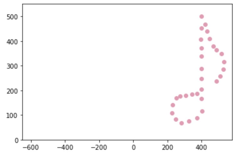

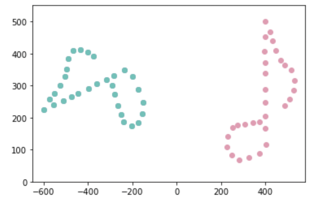
Create a matrix \(B\), which is a rotation of \(A\) with some noise. \(B\) is plotted in lavender below.

#Create B

theta = np.pi * 0.6
R_known = np.array([[np.cos(theta), -np.sin(theta)],[np.sin(theta), np.cos(theta)]])

epsilon = 0.01 # noise
B = np.dot(R_known,A) + epsilon * np.random.normal(0,1, A.shape)

#Plot
plt.scatter(A.transpose()[:,0], A.transpose()[:,1], c='#ea99b2')
plt.scatter(B.transpose()[:,0], B.transpose()[:,1], c='#8b7fa4')

plt.xlim([-650,580])
plt.ylim([0,550])

plt.show()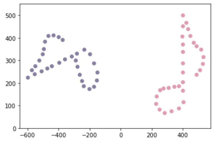

Now Orthogonal Procrustes is used to find a matrix \(R\) which will allow for a mapping from \(A\) to \(B\).

#Find orthogonal matrix

from numpy.linalg import svd

M=np.dot(B,A.transpose())
u,s,vh=svd(M)
R=np.dot(u,vh)

Transform \(A\) using \(R\) to map it to \(B\). The transformed matrix \(A_{\text{new}}=RA\).

\(A_{\text{new}}\) is plotted using cyan below: it overlaps \(B\) so closely that we can’t see the lavendar plot of B underneath.

# Mapped matrix
new_A=np.dot(R,A)

from matplotlib import pyplot as plt

plt.scatter(B.transpose()[:,0], B.transpose()[:,1], c='#8b7fa4')
plt.scatter(A.transpose()[:,0], A.transpose()[:,1], c='#ea99b2')
plt.scatter(new_A.transpose()[:,0], new_A.transpose()[:,1], c='#55c3b8')

plt.xlim([-650,580])
plt.ylim([0,550])

plt.show()