During an fMRI experiment, brain images are acquired over time while the subject is exposed to certain stimuli or performs a set of tasks. Differences in the measured signal between each scan are used to infer activation in the brain related to stimuli or task-performance. Inferences can also be made about how different parts of the brain work together or about disease states. Statistical procedures are used to make these inferences. However, modeling fMRI data is challenging because the measured signal is weak, there is a lot of noise present, and there is complex spatio-temporal correlation between different parts of the brain and successive scans. The data are also enormous. Usually 100-200 scans are taken per subject and each scan is divided into at least 100,000 parts known as voxels. The experiment may be repeated multiple times for the same subject and also for multiple subjects. It is not currently feasible to completely model the spatio-temporal dependence in fMRI data. Generally an autoregressive order 2, AR(2), temporal correlation structure is used and random field theory (RFT) correction is used to account for spatial dependence.

Using information from Dr. Lazar’s textbook The statistical analysis of functional MRI data (2008) and Dr. Lindquist’s paper The Statistical Analysis of fMRI Data (2008) to provide an introduction to understanding fMRI data and its statistical analysis.

Data Acquisition

Neural imaging using fMRI data is based on the discrepancy in magnetic resonance between oxygenated and de-oxygenated blood. Blood that is still carrying oxygen from the lungs to the brain reacts differently to a magnetic field than blood that has already released oxygen into the brain cells. Furthermore, active neurons use more oxygen than neurons that are not in use and, hence, require a greater flow of oxygenated blood. The fMRI detects increased oxygenated blood flow using magnetic fields and, thus, is able to identify areas of greater neural activation. This measurement of oxygenated blood flow is called blood-oxygen-level-dependent (BOLD) signal.

The MRI machine uses both magnetic and radio waves to detect the BOLD signal. An average MRI machine usually has a 3 tesla capacity, that is, they are able to produce magnetic waves about 50,000 times stronger than the earth’s magnetic field. The MRI scanner first targets radio waves at the protons in the area of interest. Then a magnetic field is generated which aligns the protons and then a burst of radio waves is released which knocks the protons out of alignment again. Once the radio waves cease, the protons go back in alignment with the magnetic field and in the process of realignment, the protons release a signal that the MRI scanner records.

The protons in oxygenated areas produce stronger signals than deoxygenated areas. The recorded signals are then used to create a three-dimensional image of the brain. A grid is superimposed on the brain image so neural activity can be mapped into small cubes called voxels, which are usually about 3mm x 3mm x 3mm. A typical MRI scan will consist of at least 100,000 voxels and each voxel represents thousands of neurons.

Hemodynamic response

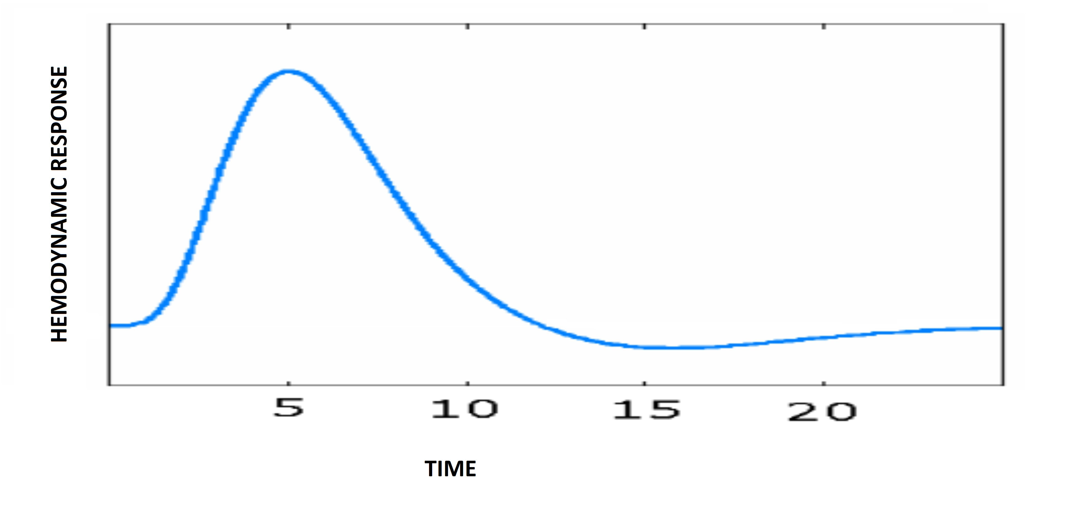
The analysis of fMRI data depends on the assumption that the measured BOLD responses correspond to the underlying neural responses, typically referred to as the hemodynamic response. Different types of brain tissue have different hemodynamic responses to activation but they all follow a similar pattern. A typical hemodynamic response to activation, known as a standard or canconical hemodynamic response function, (HRF) is shown below.

In an fMRI experiment a stimuli will not typically just be applied once but multiple times in a block or event related design. A predicted HRF for an active voxel in such an experiment can be created by convolving the canonical HRF with the design parameters. A visual example of this can be seen below.

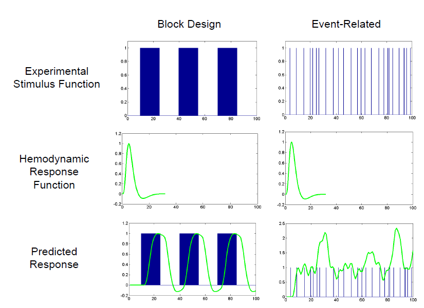
If there are multiple stimuli or tasks in an experiment then a separate predicted HRF is created for each of them. The measured BOLD response is then compared with the predicted HRF to check for voxel activation.

Noise

The MR signal usually contains many elements that are not of interest. It is important to remove or model them since the hemodynamic response is very weak. The main sources of noise in fMRI signals are system noise and physiological noise.

System noise is created by the MR hardware, mostly due to magnetic field created by the scanner drifting over time or not being spatially uniform. This type of noise should either be removed during data pre-processing or be included covariates in the statistical model. Generally two drift parameters are included during modeling to account for scanner instabilities. Physiological noise is created by head movement, breathing, heart beat, respiration, fidgeting, or making physical responses such as button presses for task related experiments. Heart beat and respiration are most often left unaccounted for though sometimes they are removed during pre-processing using filters or included as covariates in the statistical model.

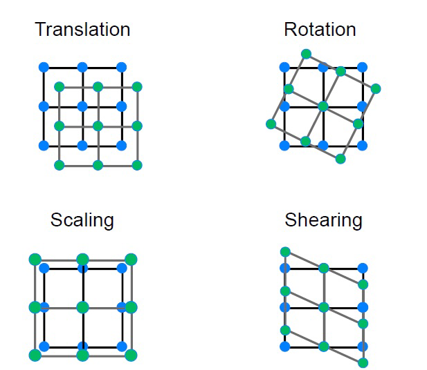
However, signal distortion due to motion is usually corrected for during pre-processing using transformations -translation, rotation, scaling, and shearing (a depiction is shown below). The motion correction parameters for each subject are then usually included as covariates in the statistical model.

Statistical Model

Common objectives of fMRI analysis are localizing regions of the brain activated by certain stimuli or tasks, identifying neural networks associated with different functions, and diagnosing disease states. All of these goals involve identifying voxel activation given specific stimuli or tasks.

Most commonly a univariate LM approach is used to identify voxel activation. A linear model is used for each voxel individually to test whether or not it is activated by the given stimuli. Assuming that the data consists of a brain volume with N voxels that is repeatedly measured at T different time points, the vector of BOLD responses from voxel i over scans 1 through T can be modeled as,

Using Dr. Lindquist’s descriptions of the statistical model in both his Coursera course and The Statistical Analysis of fMRI Data, the design matrix, X, can be partitioned into the different types of covariates used. The following is a general partitioning including all covariates that are reasonable to be included in the model.

where ,
j_T = Tx1 vector of 1’s
H = matrx of hemodynamic response functions. The number stimuli determines the number of columns.
D = matrix for the drift parameters. Most commonly two drift parameters are used, that is, this matrix has two columns.
M = matrix for the motion parameters. The number of columns will depend on the number of transformations used to correct for movement
N = matrix for the other nuisance covariates, like heart rate, respiration etc.

The covariance matrix, Vi, depends on the type of auto-correlation structure used. For example,

1. Temporal Independence. Here V_i = σ_i²I
   2. Autoregressive order 1, AR(1). Here,

      e_t,i = u_t,i + φ_iu_t-1,i ;
      t = 1,…,T;
      i = 1,…,N;
      u_t,i ~ N(0; σ_i²)

3. Autoregressive order 2, AR(2). Here,

   e_t,i = u_t,i + φ_1iu_t-1,i + φ_2iu_t-2,i;
   t = 1,…,T;
   i = 1,…,N;
   u_t,i ~ N(0; σ_i²)

   After model fitting, hypothesis tests are performed at each voxel to identify activation. For each stimulus, the null hypothesis is that the regression coefficient for its predicted HRF is zero versus the alternate hypothesis that the coefficient is greater than zero. Usually a T-statistic is used.

Example

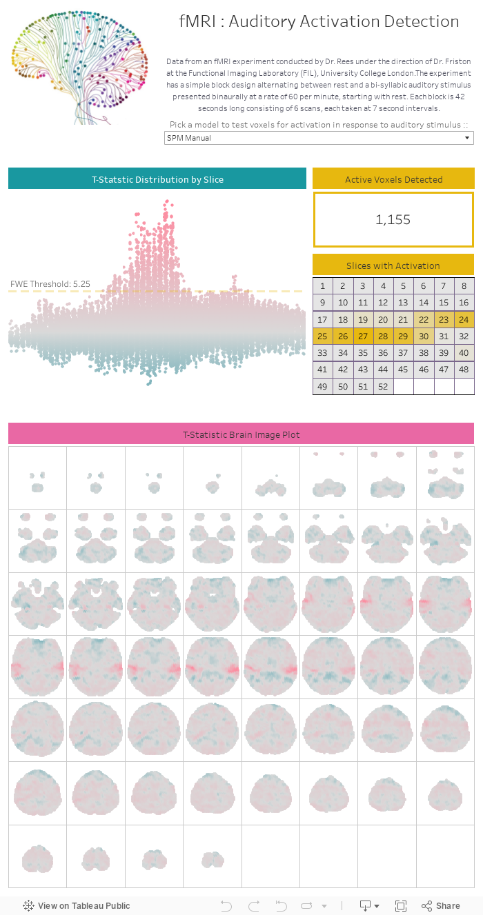
Data from an fMRI experiment conducted by Dr. Rees under the direction of Dr. Friston at the Functional Imaging Laboratory (FIL), University College London were used. The purpose of the experiment was equipment testing and creating a dataset for educational purposes, which is our purpose as well. The experiment consists of whole brain 3D images from 96 scans, each divided into a 64x64x64 grid, that is, 262144 voxels. Each voxel is 3mm x 3mm x 3mm.

The experiment has a simple block design alternating between rest and a bi-syllabic auditory stimulus presented binaurally at a rate of 60 per minute, starting with rest. Each block is 42 seconds long consisting of 6 scans, each taken at 7 second intervals. The change in BOLD contrast from each voxel is measured. The purpose of our analysis is to determine which voxels are activated by the auditory stimulus.

Preprocessing is done using SPM in Matlab. Steps from the SPM Manual are followed. Animation of the signal across the 96 scans across each slice after preprocessing is shown below :

To detect voxels activated by the auditory stimulus, a few different models are fit to the preprocessed data:

• SPM Manual Default Model
• No autocorrelation (temporal independence) with motion parameters (R)
• No autocorrelation (temporal independence) without motion parameters (R)
• AR1 autocorrelation with motion parameters (R)
• AR1 autocorrelation without motion parameters (R)

Using each model, T-Statistics are calculated for each voxel. The familywise error (FWE) Threshold from SPM is used to correct for multiple hypothesis testing. The Test Statistics can be found below :

            <script type='text/javascript'>                    var divElement = document.getElementById('viz1539057915945');                    var vizElement = divElement.getElementsByTagName('object')[0];                    vizElement.style.width='700px';vizElement.style.height='1327px';                    var scriptElement = document.createElement('script');                    scriptElement.src = 'https://public.tableau.com/javascripts/api/viz_v1.js';                    vizElement.parentNode.insertBefore(scriptElement, vizElement);                </script></div>